1. Scaling
<스케일링 클래스>
StandardScaler() : 평균이 0, 표준편차가 1이 되도록 정규화
RobustScaler(): 중강값이 0, IQR(interquartile range)이 1이 되도록 스케일링
MinMaxScaler() : 최대값이 1, 최소값이 0이 되도록 스케일링
MaxAbsScaler() : 0을 기준으로 절대값이 가장 큰 수가 1 또는 -1이 되도록 스케일링
<주요 메서드>
fit: 분포 모수를 객체 내에 저장
transform: 학습용 데이터를 입력하여 저장된 분포 모수를 이용해서 데이터를 스케일링
fit_transform: fit-transform을 합쳐서 한번에 이용

from sklearn.preprocessing import MinMaxScaler

scaler = MinMaxScaler()
scaler.fit(data)
scaled_data = scaler.transform(data) #numpy 배열 반환

scaled_data = pd.DataFrame(scaled_data, colums = data.columns)
scaled_data.head()
2. sampling
클래스 불균형 : 분류를 목적으로하는 데이터 셋에 클래스 라벨의 비율 균형이 맞지 않는 경우.
<random oversampling & random undersampling>
oversampling : 적은 클래스의 데이터 수를 증가시키는 것
undersampling : 많은 클래스의 데이터 수를 감소시키는 것
Random__Sampler()객체의 fit_resample 메서드로 샘플링된 데이터와 라벨을 리턴해준다.
from imblearn.over_sampling import RandomOverSampler
from imblearn.under_sampling import RandomUnderSampler

ros = RandomOverSampler()
rus = RandomUnderSampler()

oversampled_data, oversampled_label = ros.fit_resample(data, label)
oversampled_data = pd.DataFrame(oversampled_data, columns = data.columns)

undersampled_data, undersampled_label = rus.fit_resample(data, label)
undersampled_data = pd.DataFrame(undersampled_data, columns = data.columns)
print('원본 데이터의 클래스 비율 \n{}'.format(pd.get_dummies(label).sum()))
print('\nRandom over 샘플링 결과 \n{}'.format(pd.get_dummies(oversampled_label).sum()))
print('\nRandom under 샘플링 결과 \n{}'.format(pd.get_dummies(undersampled_label).sum()))
#원본 데이터의 클래스 비율
#F 1307
#I 1342
#M 1528
#dtype: int64
#
#Random over 샘플링 결과
#F 1528
#I 1528
#M 1528
#dtype: int64
#
#Random under 샘플링 결과
#F 1307
#I 1307
#M 1307
#dtype: int64(get_dummies의 사용은 suuntree.tistory.com/269참고)
random over sampling은 단순히 적은 라벨 갖는 데이터를 무작위로 선택하여 복제하는 식으로 샘플링을 한다.
-> 해당 데이터에 과대적합 될 수 있다.
random under sampling은 단순히 많은 라벨을 갖는 데이터를 무작위로 선택하여 삭제하는 식으로 샘플링을 한다.
-> 데이터 손실이 크다.
<SMOTE>
smote(synthetic minority oversampling technique) : 기본적으로 oversampling이다.
임의의 한 데이터를 골라서 k개의 최근접 이웃들의 무게중심이 되는 데이터를 만든다. 과대적합을 줄일 수 있다.
make_classification함수로 1000개의 샘플, 2차원, 3개의 클래스를 갖는 데이터를 생성해준다. 세가지 라벨은 5:15:80비율로 생성한다.
from sklearn.datasets import make_classification

data, label = make_classification(n_samples = 1000, n_features=2, n_informative=2,
                                 n_redundant=0, n_repeated=0, n_classes=3,
                                 n_clusters_per_class=1,
                                 weights=[0.05, 0.15, 0.8],
                                 class_sep=0.8, random_state=2019)
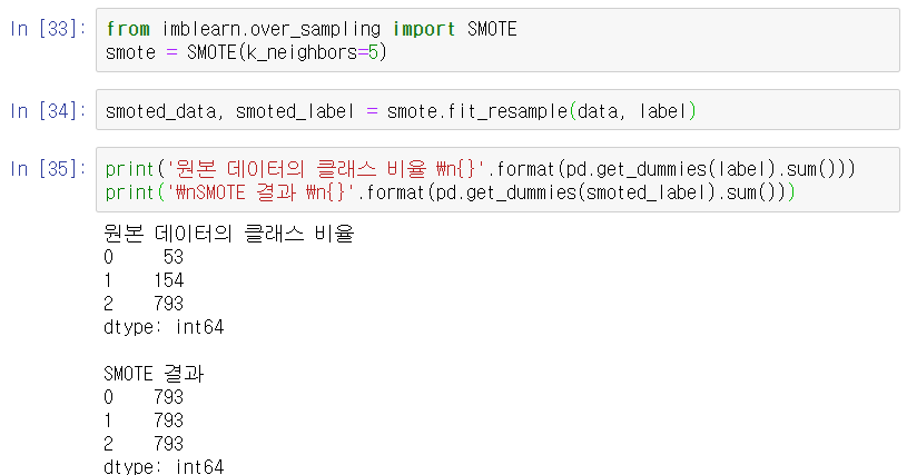
선택된 점마다 5개의 최근접 이웃의 무게중심이 되는 데이터를 생성하도록 하는 SMOTE 샘플러 객체를 만들어서 샘플링한다.

3. PolynomialFeatures
데이터가 비선형인 경우, 각 특성을 n차 다항하여 새로운 특성으로 추가하는 모듈.
확장된 특성을 포함한 데이터로 선형 모델을 훈련시키면 데이터가 비선형이더라도 훈련 가능하다.

위 데이터로 다항회귀를 수행할 것.
직선은 이 데이터에 잘 맞지 않을 것이므로 사이킷런의 PolynomialFeatures를 사용해 훈련 데이터를 변환 후 회귀 수행
from sklearn.preprocessing import PolynomialFeatures

poly_features = PolynomialFeatures(degree=2, include_bias = False)
X_poly = poly_features.fit_transform(X)
X[0]	#array([-0.75275929])
X_poly[0]	#array([-0.75275929,  0.56664654])


# include_bias = True, 편향을 위한 특성 1
#linearregression 모델이 model.intercept_, model.coef_ 알아서 구해줌
# 편향을 위한 특성 x_0 없이 사용
polynomialfeatures이 특성을 어떻게 확장했는지 get_feature_names()로 확인할 수 있다.
poly_features.get_feature_names()
# ['x0', 'x0^2']
확장된 데이터로 선형모델 학습한다.
lin_reg = LinearRegression()
lin_reg.fit(X_poly,y)
lin_reg.intercept_, lin_reg.coef_
#(array([1.78134581]), array([[0.93366893, 0.56456263]]))
실제 함수가 $y = 0.5x_1^{2} + 1.0x_1+2.0+noise$이고 예측된 모델은 $\hat{y} = 0.56x_1^{2} + 0.93x_1+1.78$이다.
4. OrdinalEncoder
어떤 특성을 범주형 특성으로 간주해서 숫자로 바꾸는 클래스

위와 같은 특성을 숫자로 인코딩하는 것
from sklearn.preprocessing import OrdinalEncoder

ordinal_encoder = OrdinalEncoder()
housing_cat_encoded = ordinal_encoder.fit_transform(housing_cat)
housing_cat_encoded[:5]
#array([[0.],
#       [0.],
#       [4.],
#       [1.],
#       [0.]])
4. OneHotEncoder
어떤 특성을 범주형 특성으로 간주해서 one-hot encoding하는 클래스.
ordinal encoding은 2와 3이 가깝다고 생각하기 때문에 부적절한 경우가 많다.
scipy의 희소행렬로 만들어주기 때문에 toarray로 변환해야 한다.
from sklearn.preprocessing import OneHotEncoder

cat_encoder = OneHotEncoder()
housing_cat_1hot = cat_encoder.fit_transform(housing_cat)

print(type(housing_cat_1hot)) #<class 'scipy.sparse.csr.csr_matrix'>
housing_cat_1hot.toarray()
#array([[1., 0., 0., 0., 0.],
#       [1., 0., 0., 0., 0.],
#       [0., 0., 0., 0., 1.],
#       ...,
#       [0., 1., 0., 0., 0.],
#       [1., 0., 0., 0., 0.],
#       [0., 0., 0., 1., 0.]])
categories_속성으로 카테고리 확인 가능
cat_encoder.categories_
#[array(['<1H OCEAN', 'INLAND', 'ISLAND', 'NEAR BAY', 'NEAR OCEAN'],
# dtype=object)]'ML&DATA > ML' 카테고리의 다른 글
| sklearn - impute (0) | 2020.10.02 |
|---|---|
| sklearn - model_selection (0) | 2020.10.02 |
| sklearn - pipeline, compose (0) | 2020.09.01 |
| sklearn - make_classification (0) | 2020.09.01 |
