어떤 데이터의 라벨이 양자화된 값들로 결정되는 경우 multinomial classification으로 새로운 input데이터의 라벨을 예측하는 방법.
#label 번의 binary classification을 수행하여 라벨마다 확률을 구해준 후 가장 큰 확률을 갖는 라벨을 output으로 예측하는 방법이다.
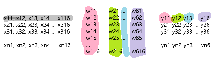
#label번의 binary classification을 수행하기 위해 가중치 벡터를 이어붙인 가중치 매트릭스를 사용한다.
설명의 편의를 위해 $f(X) = XW+b$ 대신 다음 링크함수를 사용한다. $$f(X) = WX$$

bias는 어디있고 XW가 아닌 WX를 사용하는 이유가 뭔지?
XW+B를 다르게 표현하면 X*W+1*B로 나타낼 수 있기때문에 1을 X의 벡터 첫번째 항으로 추가시켜주고, B를 W의 첫번째 항으로 추가시켜줍니다. 즉 X = [1 X1 X2 ... Xn], W = [B W1 W2 ...Wm] 이렇게 나타낼 수 있기때문에 이전의 식을 XW로 간단하게 표현할 수 있습니다.
(https://www.youtube.com/watch?v=MFAnsx1y9ZI&list=PLQ28Nx3M4Jrguyuwg4xe9d9t2XE639e5C&index=12)댓글
위 그림의 결과 [[y1], [y2], [y3]]를 sigmoid에 넣지 않고, softmax함수를 사용한다.
$$S(y_i) = \frac{e^{y_i}}{\sum{}{}e^{y_j}}$$
(단순히 전체에 대한 해당 값의 비율이 아닌 위와같은 softmax함수를 쓰는 건 예측함수의 비선형성을 위함이라고 함)
softmax함수의 출력값과 실제 값(라벨 값)으로 cross entropy함수를 정의할 수 있다. (비용함수에 사용함)
i번째 데이터에 대한 cross entropy $D(S_i, L_i)$는 다음과 같다.
$$D(S_i, L_i) = -\sum_{j}^{num \, of\, label}L_j\, log\, S_j$$
비용함수는 다음과 같다
$$cost = \frac{1}{m}\sum_{i}D(S(X_iW+b), L_i)$$
cross entropy와 logistic cost는 본질적으론 같다. 더보기에서 확인하자.

라벨이 2가지인 경우 binary classification의 결과는 0또는 1인 반면, multinomial classification의 결과는 [1,0] 또는 [0,1]이다.
L2 = 1-L1이라고 할 수 있고 s2 = 1-s1이라고 할 수 있다.
cross entropy를 위 식으로 전개해보면 다음과 같다.
$$D(S,L) = -L_1log(S_1) - L_2log(S_2)$$
$$D(S,L) = -L_1log(S_1) - (1-L_1)log(1-S_1)$$
따라서 라벨이 2가지인 경우 logisitic cost와 cross entropy는 같다.
cross entropy는 logistic cost를 확장시킨 개념이라고 할 수 있겠다.
가설함수와 비용함수
$$H(X) = S(XW+b)$$
$$cost = \frac{1}{m}\sum_{i}D(S(X_iW+b), L_i)$$
hypothesis = tf.nn.softmax(tf.matmul(features,W)+b)
cost = tf.reduce_mean(-tf.reduce_sum(y_data * tf.math.log(hypothesis), axis=1))
tf.nn.softf.nn.softmax_cross_entropy_with_logit을 이용한 비용함수. 가설함수가 아닌 로짓을 사용함에 주의
def logit_fn(X):
    return tf.matmul(X,W)+b

def cost_fn(X,Y):
    logits = logit_fn(X)
    cost_i = tf.nn.softmax_cross_entropy_with_logits(logits = logits, labels = Y)
    cost = tf.reduce_mean(cost_i)
    return cost
<csv파일을 이용한 실습>
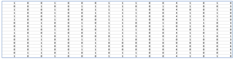
16개의 feature가 7개 class 중 하나의 label을 결정하는 데이터를 이용한 multinomial classification
import tensorflow as tf
import numpy as np

xy = np.loadtxt('data-04-zoo.csv', delimiter = ',', dtype = np.float32)
x_data = xy[:,0:-1]
y_data = xy[:,[-1]].astype(np.int32)
csv파일로부터 데이터를 읽어와서 feature와 label을 분류한다. 이때 label이 0~6값을 갖는데, multinomial classification을 위해 one_hot 형식으로 바꾸는 전처리가 필요하다.
y_data를 category variable로 사용할것이므로 int로 형변환이 필요하다. (안하면 에러)
nb_classes = 7
Y_one_hot = tf.one_hot(list(y_data), nb_classes)
Y_one_hot = tf.reshape(Y_one_hot, [-1, nb_classes])
y_data는 2차원 리스트인데 tf.one_hot을 적용하면 차원이 하나 늘어서 3차원이 된다.
tf.reshape하여 2차원으로 만들어줘야 한다.

W = tf.Variable(tf.zeros([16, nb_classes]), name = 'weight')
b = tf.Variable(tf.zeros([nb_classes]), name = 'bias')
variables = [W,b]
가중치 matrix와 bias를 랜덤값으로 초기화해준다. 아래 그림에 맞게 차원을 맞춰줘야 함
def logit_fn(X):
return tf.matmul(X,W)+b
def hypothesis(X):
return tf.nn.softmax(logit_fn(X))
def cost_fn(X,Y):
logits = logit_fn(X)
cost_i = tf.nn.softmax_cross_entropy_with_logits(logits = logits, labels = Y)
cost = tf.reduce_mean(cost_i)
return cost
def grad_fn(X,Y):
with tf.GradientTape() as tape:
loss = cost_fn(X,Y)
grads = tape.gradient(loss, variables)
return grads
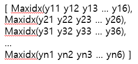
def prediction(X,Y):
pred = tf.argmax(hypothesis(X), 1)
correct_prediction = tf.equal(pred, tf.argmax(Y,1))
accuracy = tf.reduce_mean(tf.cast(correct_prediction, tf.float32))
return accuracy 적절히 함수들 정의
prediction(X,Y): (W,b)를 이용한 가설함수가 X,Y에 대해 동작하는 정확성 출력
위에 그림에서 색칠한 결과가 hypothesis(X)에 해당.
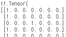
pred는 다음과 같음. 1차원 리스트가 담긴 텐서임
tf.argmax(Y,1)은 라벨에서 1이 있는 인덱스임. correct_prediction은 pred와 tf.argmax(Y,1)의 원소 하나씩 비교해서 같으면 1 다르면 0(boolean)을 리스트에 저장. -> correct_prediction도 1차원 리스트
correct_prediction은 boolean type이므로 tf.float32으로 cast후에 평균을 구하면 예측이 맞은 횟수의 확률, 즉 정확도를 구할 수 있다.
def fit(X, Y, epochs=500, verbose = 50):
    optimizer = tf.keras.optimizers.SGD(learning_rate = 0.01)
    for i in range(epochs):
        grads = grad_fn(X,Y)
        optimizer.apply_gradients(zip(grads, variables))
        if (i==0) | ((i+1)%verbose==0):
            acc = prediction(X,Y).numpy()
            loss = tf.reduce_sum(cost_fn(X,Y)).numpy()
            print("Loss & Acc at {} epoch {}, {}".format(i+1, loss, acc))

fit(x_data, Y_one_hot)
전처리한 데이터 x_data와 Y_one_hot으로 fit(가중치 matrix를 조정)하는 코드.
전체코드
import tensorflow as tf
import numpy as np

xy = np.loadtxt('data-04-zoo.csv', delimiter = ',', dtype = np.float32)
x_data = xy[:,0:-1]
y_data = xy[:,[-1]].astype(np.int32)

nb_classes = 7
Y_one_hot = tf.one_hot(list(y_data), nb_classes)
Y_one_hot = tf.reshape(Y_one_hot, [-1, nb_classes])

W = tf.Variable(tf.zeros([16, nb_classes]), name = 'weight')
b = tf.Variable(tf.zeros([nb_classes]), name = 'bias')
variables = [W,b]

def logit_fn(X):
    return tf.matmul(X,W)+b

def hypothesis(X):
    return tf.nn.softmax(logit_fn(X))

def cost_fn(X,Y):
    logits = logit_fn(X)
    cost_i = tf.nn.softmax_cross_entropy_with_logits(logits = logits, labels = Y)
    cost = tf.reduce_mean(cost_i)
    return cost

def grad_fn(X,Y):
    with tf.GradientTape() as tape:
        loss = cost_fn(X,Y)
        grads = tape.gradient(loss, variables)
        return grads

def prediction(X,Y):
    pred = tf.argmax(hypothesis(X), 1)
    correct_prediction = tf.equal(pred, tf.argmax(Y,1))
    accuracy = tf.reduce_mean(tf.cast(correct_prediction, tf.float32))
    return accuracy

def fit(X, Y, epochs=500, verbose = 50):
    optimizer = tf.keras.optimizers.SGD(learning_rate = 0.01)
    for i in range(epochs):
        grads = grad_fn(X,Y)
        optimizer.apply_gradients(zip(grads, variables))
        if (i==0) | ((i+1)%verbose==0):
            acc = prediction(X,Y).numpy()
            loss = tf.reduce_sum(cost_fn(X,Y)).numpy()
            print("Loss & Acc at {} epoch {}, {}".format(i+1, loss, acc))

fit(x_data, Y_one_hot)
'ML&DATA > 모두를 위한 딥러닝' 카테고리의 다른 글
| 실습 (0) | 2020.07.13 |
|---|---|
| application & tips (0) | 2020.07.13 |
| binary classification (0) | 2020.07.10 |
| simple linear regression (단순 선형 회귀) (0) | 2020.07.08 |
| 용어/개념 (0) | 2020.07.08 |


